
November 2006 B
|
Designing Scalable Synthetic Compact Applications for Benchmarking High Productivity Computing Systems
|
 November 2006 B |
One of the main objectives of the DARPA High Productivity Computing Systems (HPCS) program is to reassess the way we define and measure performance, programmability, portability, robustness and ultimately productivity in the High Performance Computing (HPC) domain. This article describes the Scalable Synthetic Compact Applications (SSCA) benchmark suite, a community product delivered under support of the DARPA HPCS program. The SSCA benchmark suite consists of six benchmarks. The first three SSCA benchmarks are specified and described in this article. The last three are to be developed and will relate to simulation. SSCA #1 Bioinformatics Optimal Pattern Matching stresses integer and character operations (no floating point required) and is compute-limited; SSCA #2 Graph Analysis stresses memory access, uses integer operations, is compute-intensive, and is hard to parallelize on most modern systems; and SSCA #3 Synthetic Aperture Radar Application is computationally taxing, seeks a high rate at which answers are generated, and contains a significant file I/O component. These SSCA benchmarks are envisioned to emerge as complements to current scalable micro-benchmarks and complex real applications to measure high-end productivity and system performance. They are also described in sufficient detail to drive novel HPC programming paradigms, as well as architecture development and testing. The benchmark written and executable specifications are available from www.highproductivity.org.
One of the main objectives of the DARPA High Productivity Computing Systems (HPCS) program1 is to reassess the way we define and measure performance, programmability, portability, robustness and ultimately productivity in the High Performance Computing (HPC) domain. An initiative in this direction is the formulation of the Scalable Synthetic Compact Applications (SSCA)2 benchmark suite. Each SSCA benchmark is composed of multiple related kernels which are chosen to represent workloads within real HPC applications and is used to evaluate and analyze the ease of use of the system, memory access patterns, communication and I/O characteristics. The benchmarks are relatively small to permit productivity testing and programming inreasonable time; and scalable in problem representation and size to allow simulating a run at small scale or executing on a large system at large scale.
Each benchmark written specification presents detailed background and parameters for an untimed data generator and a number of timed application kernels. All of the SSCA benchmarks are intended to be scalable using any of a variety of techniques, a variety of languages, and a variety of machine architectures. Each SSCA includes a number of untimed validation steps to provide checks an implementor can make to gain confidence in the correctness of the implementation.
The SSCA benchmark suite consists of six benchmarks. The first three SSCA benchmarks are specified and described in this article. The last three are to be developed and will relate to simulation.
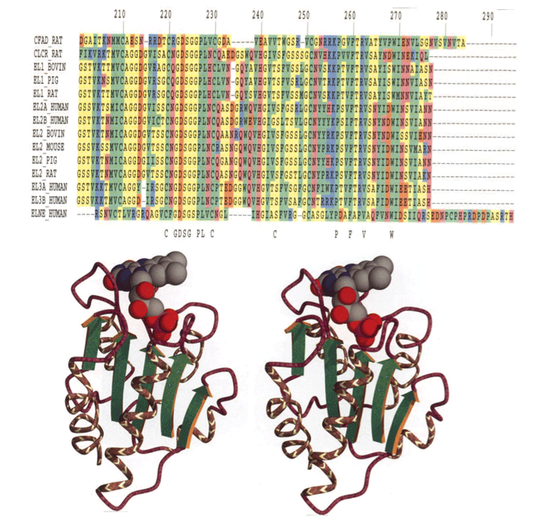
The intent of this SSCA is to develop a set of compact application kernels that perform a variety of analysis techniques used for optimal pattern matching. The chosen application area is from an important optimization problem in bioinformatics and computational biology, namely, aligning genomic sequences. These references provide an introduction to the extensive literature on this problem space, some publicly available programs that address these problems, and the algorithms used in those programs: 3 4 5 6 7 8 9 10 11 12 13 14
A genome consists of a linear sequence composed of the four deoxyribonucleic acid (DNA) nucleotides (bases), which forms the famous double helix. The DNA sequence contains the information needed to code the proteins that form the basis for life. Proteins are linear sequences of amino acids, typically 200-400 amino acids in length. Each different protein twists naturally into a specific, complex 3-dimensional shape. This shape is what primarily determines the protein’s function.
Three adjacent DNA bases form each of 64 different codons, 61 of which code for the 20 different amino acids, while the three remaining codons indicate a stop to the coding region for the current protein. A particular amino acid may have from one to six different encodings.
Different organisms typically use similar proteins for similar purposes. A slight change in the amino acid sequence can cause anything from a slight to a profound change in the shape of the resulting protein. A slight change in the DNA sequence can cause anything from no change to a profound change in the amino acid sequence. Profound changes are almost always bad for the organism, but smaller changes may be good, bad, or neutral. Such changes (mutations) are continually occurring as a result of radiation, chemical agents, copying errors, etc.
Mutations can change individual bases, or can add or delete sections of DNA. Adding or deleting individual bases almost always produces a profound change, but adding or deleting a sequence of 3n bases may have only a slight effect since the subsequent amino acids remain unchanged.
Automated techniques have produced enormous libraries of DNA sequences identified by organism. Laboratory research has produced enormous libraries of protein sequences identified by organism and function. Today, much biological research depends on finding and evaluating approximate matches between sequences from these libraries.
In this SSCA, we consider the polynomial time problem of pairwise sequence alignment and the potentially NP-hard problem of multiple sequence alignment. Algorithms that solve these problems are often integer-based and use a variety of algorithmic techniques and heuristics. Optimal algorithms exist and are practical for pairwise alignment. However, approximate or heuristic algorithms are required for multiple sequence alignment; there is no single, obviously best approach to the problem, and the simple algorithms are either NP-hard or approximations.
In biology, multiple sequence alignments are needed to:
No one alignment algorithm is suitable for all these applications, but most commonly used alignment programs use variants of a single basic approach, the dynamic programming algorithm for optimal pairwise sequence alignment. The kernels below explore several of these variations.
The first kernel performs a local pairwise alignment of two long codon sequences, finding the end-points of subsequences that are good matches according to the specified criteria. The second kernel identifies actual codon sequences located by the first kernel, working backward from the given end-points. The third kernel uses the interesting subsequences found in the second sequence by the second kernel to search the first sequence for a set of the best complete matches to each interesting subsequence. The fourth kernel goes through each set of matches found by the third kernel and performs a global pairwise alignment at the nucleotide level for each pair. The fifth kernel performs multiple sequence alignment on each of the sets of alignments generated by the third kernel, using the simple, approximate “center star” algorithm.
This SSCA requires a scalable data generator to create genomic sequences of lengths from hundreds to potentially billions of nucleotide bases. At least four types of data are commonly used for sequence matching: DNA, RNA, codons, and amino acids.
Usually the division of DNA/RNA into codons is known, and matching at the codon level is the most informative and fastest. Matching at the nucleotide level is interesting for some applications, but is much slower. Matching at the amino acid level is important only if the corresponding DNA/RNA is unknown, and uses almost exactly the same algorithms as codon-level matching. For this SSCA we have chosen to specify DNA codon-level pairwise alignment and DNA nucleotide-level multiple sequence alignment.
Waterman14 states: “Surprising relationships have been discovered between sequences that overall have little similarity. These are dramatic cases when unexpectedly long matching segments have been located between viral and host DNA. [Smith-Waterman] is a dynamic programming algorithm to find these segments. This is probably the most useful dynamic programming algorithm for current problems in molecular biology. These alignments are called local alignments.” For this first kernel, we are given two sequences and wish to find the subsequences from these two that are most similar to each other as defined by Waterman. There may be several ‘equally similar’ subsequence pairs.
Using the end-point pairs and similarity scores produced by kernel 1, kernel 2 locates actual subsequence pairs with those scores. If there is more than one match for a particular end-point pair, only the best one should be reported. This kernel is specified separately from kernel 1, since keeping track of the actual sequences in kernel 1 would require some extra computation and perhaps a great deal of extra space.
For the second of each pair of subsequences produced by kernel 2, remove any gaps and search the first full sequence for the 100 best matches to the entire compacted subsequence.
The result of kernel 4 is 100 sets of 100 highly similar subsequences, taken from the first of the two original full sequences.
For each of these sets, this kernel prepares the way for the kernel 5 multiple-sequence alignment algorithm by aligning each pair of subsequences and reporting their alignment score. The scoring algorithm does global matching using a scoring function, which operates at the nucleotide level and does not include any gap-start penalty. Instead of measuring similarity directly, it measures differences between the strings, so computing optimal alignments requires minimizing the difference-score rather than maximizing a similarity score.
The result of kernel 4 is 100 sets of 100 subsequences, pairwise aligned and scored for similarity at the nucleotide level. Kernel 5 then arranges each set of subsequences into a multiple alignment that approximates an alignment, which might be of interest to someone studying relationships between the subsequences within each set.
A Multiple Sequence Alignment (MSA) is defined as follows. A multiple alignment of strings S[1], . . . , S[k] is a series of strings S'[1], . . . , S'[k] with spaces (internal gaps), such that the new sequences S'[] are all of the same length n, and S'[j] is an extension of S[j] by insertion of spaces for 1 ≤ j ≤ k find an optimal multiple alignment.
For biological purposes an optimal multiple alignment is one which most clearly shows the relationships of the various sequences. These relationships may be evolutionary and/or structural, and may depend on additional data such as known kinship relationships or 3-dimensional protein shape correlations. Many different approaches are possible and this remains an active research area.
Sum-of-Pairs (SP) is one simple theoretical measure of multiple alignment. Given a specific multiple alignment (including spaces), the global similarity of each pair of sequences is calculated separately. The sum of these pairwise similarities is the SP measure. The minimum of SP over all possible multiple alignments is the theoretically optimal SP alignment.
Finding the optimal SP alignment is NP-hard; using dynamic programming it runs in O(k22knk) time, that is, exponential in the number of sequences. For n = 200 and k = 100, this is prohibitive. A number of different approximate methods are known, of varying performance, quality, and complexity, such as the Star, Tree, and various Progressive alignments. Star alignment runs in polynomial time, but the result can be far from optimal. Tree alignment maps the k sequences to a tree with k leaves, is NP-complete, and requires a tree selection heuristic.
Progressive alignments (such as ClustalW, PileUp, or T-Coffee) are perhaps the most practical and widely used methods, and are a hierarchical extension of pairwise alignments. They compare all sequences pairwise, perform cluster analysis on the pairwise data to generate a hierarchy for alignment (guide tree), and then build the alignment step by step according to the guide tree. The multiple alignment is built by first aligning the most similar pair of sequences, then adding another sequence or another pairwise alignment.
Progressive alignments often work well for similar sequences but are problematic for distantly-related sequences. Probabilistic methods are emerging, such as HMMER,5 that perform Profile Hidden Markov Models introduced by Gribskov.6 A profile HMM can be trained from unaligned sequences, if a trusted alignment is not yet known. HMMs have a consistent theory behind gap and insertion scores, and are useful in determining protein families. Many new MSA heuristics have been published in the last few years, including techniques such as MACAW, Clustal W, DIAlign, T-Coffee, and POA.
Multiple sequence alignment is a difficult problem; as described the best solutions are either very slow or very complex. For the purposes of this SSCA we choose the "center star" approximation method, as discussed in[8], a simple example of a progressive alignment. When used with an alphabet-weighted scoring scheme that satisfies the triangle inequality, this method produces a sum-of-pairs solution that is within a factor of two of optimal (and is usually much better).
Graph theoretic problems are representative of fundamental computations in traditional and emerging scientific disciplines like scientific computing and computational biology, as well as applications in national security. This synthetic benchmark consists of four kernels that require irregular access to a large directed and weighted graph.
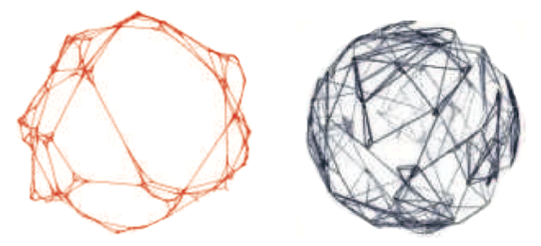
SSCA #2 is a graph theoretic problem which is representative of computations in the fields of national security, scientific computing, and computational biology. The HPC community currently relies excessively on single-parameter microbenchmarks like LINPACK,15 which look solely at the floating-point performance of the system, given a problem with high degrees of spatial and temporal locality. Graph theoretic problems tend to exhibit irregular memory accesses, which leads to difficulty in partitioning data to processors and in poor cache performance. The growing gap in performance between processor and memory speeds, the memory wall, makes it challenging for the application programmer to attain high performance on these codes. The onus is now on the programmer and the system architect to come up with innovative designs.
The intent of this SSCA is to develop a compact application that has multiple analysis techniques (multiple kernels) accessing a single data structure representing a weighted, directed graph. In addition to a kernel to construct the graph from the input tuple list, there are three additional computational kernels to operate on the graph. Each of the kernels requires irregular access to the graphs data structure, and it is possible that no single data layout will be optimal for all four computational kernels.
Two versions of this SSCA #2 have been specified. The earlier versions (1.0 and 1.1) used a different data generator and graph algorithm for kernel 4. Here we describe the latest version (2.0) and refer the reader to [16 17 18] for details on the older version 1.1.
SSCA #2 includes a scalable data generator that produces edge tuples containing the start vertex, end vertex, and weight for each directed edge. The first kernel constructs the graph in a format usable by all subsequent kernels. No subsequent modifications are permitted to benefit specific kernels. The second kernel extracts edges by weight from the graph representation and forms a list of the selected edges. The third kernel extracts a series of subgraphs formed by following paths of a specified length from a start set of initial vertices. Kernel 3’s set of initial vertices are determined by kernel 2. The fourth kernel computes a centrality metric that identifies vertices of key importance along shortest paths of the graph.
The scalable data generator constructs a list of edge tuples containing vertex identifiers, and randomly-selected positive integers are assigned as weights on the edges of the graph. Each edge is directed from the first vertex of its tuple to the second. The generated list of tuples must not exhibit any locality that can be exploited by the computational kernels. For generating the graphs, we use a synthetic graph model that matches the topologies seen in real-world applications: the Recursive MATrix (R-MAT) scale-free graph generation algorithm.19 For ease of discussion, the description of this R-MAT generator uses an adjacency matrix data structure; however, implementations may use any alternate approach that outputs the equivalent list of edge tuples. The R-MAT model recursively sub-divides the adjacency matrix of the graph into four equal-sized partitions and distributes edges within these partitions with unequal probabilities. Initially, the adjacency matrix is empty and edges are added one at a time. Each edge chooses one of the four partitions with probabilities a, b, c, and d, respectively. At each stage of the recursion, the parameters are varied slightly and renormalized. For simplicity in this SSCA, multiple edges, self-loops, and isolated vertices, may be ignored in the subsequent kernels. The algorithm also generates the data tuples with high degrees of locality. Thus, as a final step, vertex numbers must be randomly permuted, and then edge tuples randomly shuffled.
This kernel constructs the graph from the data generator output tuple list. The graph can be represented in any manner, but cannot be modified by subsequent kernels. The number of vertices in the graph is not provided and needs to be determined in this kernel.
The intent of this kernel is to examine all edge weights to determine those vertex pairs with the largest integer weight. The output of this kernel will be an edge list, S, that will be saved for use in the following kernel.
Starting from vertex pairs in the set S, this kernel produces subgraphs that consist of the vertices and edges along all paths of length less than subGrEdgeLength, an input parameter. A possible algorithm for graph extraction is Breadth-First Search.
This kernel identifies the set of vertices in the graph with the highest betweenness centrality score. Betweenness Centrality is a shortest paths, enumeration-based centrality metric introduced by Freeman.20 This is done using a betweenness centrality algorithm that computes this metric for every vertex in the graph. Let σst denote the number of shortest paths between vertices s and t, and σst(v) denote the number of paths passing through v. Betweenness centrality of a vertex v is defined as  . The output
of this kernel is a betweenness centrality score for each vertex in the graph and the set of vertices with the highest betweenness centrality score.
For kernel 4, we filter out a fraction of edges using a filter described in the written specification. Because of the high computation cost of kernel 4, an exact implementation considers all vertices as starting points in the betweenness centrality metric, while an approximate implementation uses a subset of starting vertices (VS).
A straightforward way of computing betweenness vertex would be as follows:

Recently, Brandes21 proposed a faster algorithm that computes the exact betweenness centrality score for all vertices in the graph. Brandes noted that it is possible to augment Dijkstra’s single-source shortest paths (SSSP) algorithm (for weight graphs) and breadth-first search (BFS) for unweighted graphs to compute the dependencies. Bader and Madduri give the first parallel betweenness centrality algorithm in [22].
In order to compare the performance of SSCA #2 Version 2.x kernel 4 implementations across a variety of architectures, programming models, and productivity languages and frameworks, as well as normalizing across both exact and approximate implementations, we adopt a new performance metric, a rate called traversed edges per second (TEPS).
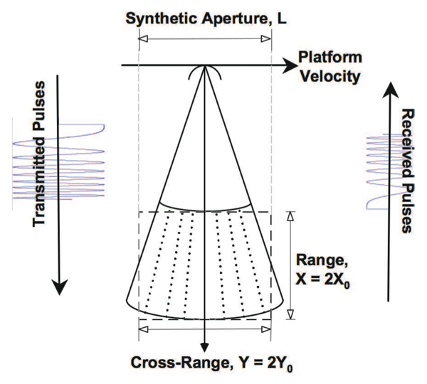
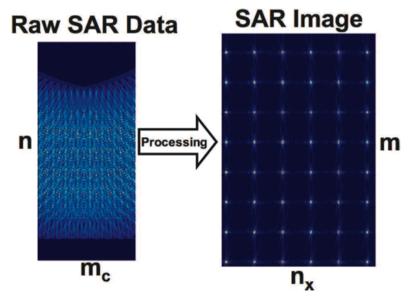
Synthetic Aperture Radar (SAR) is one of the most common modes in a RADAR system and one of the most computationally stressing to implement. The goal of a SAR system is usually to create images of the ground from a moving airborne RADAR platform. The basic physics of a SAR system begins with the RADAR sending out pulses of radio waves aimed at a region on the ground that it usually perpendicular to the direction of motion of the platform (see Fig. 3). The pulses are reflected off the ground and detected by the RADAR. Typically the area of the ground that reflects a single pulse is quite large and an image made from this raw unprocessed data is very blurry (see Fig. 4). The key concept of a SAR system is that it moves between each pulse, which allows multiple looks at the same area of the ground from different viewing angles. Combining these different viewing angles together produces a much sharper image (see Fig. 4). The resulting image is as sharp as one taken from a much larger RADAR with a “synthetic” aperture the length of the distance traveled by the platform.
There are many variations on the mathematical algorithms used to transform the raw SAR data into a sharpened image. SSCA #3 focuses on the variation referred to as “spotlight” SAR. Furthermore, SSCA #3 is a simplified version of this algorithm that focuses on the most computationally intensive steps of SAR processing that are common to nearly all SAR algorithms.
The overall block diagram for this benchmark is shown in Fig. 5 At the highest level it consists of three stages:
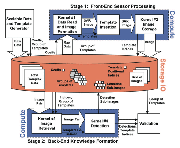
SDG: Scalable Data Generator. Creates raw SAR inputs and writes them to files to be read in by Stage 1.
Stage 1: Front-End Sensor Processing. Reads in raw SAR inputs, turns them into SAR images, and writes them out to files.
Stage 2: Back-End Knowledge Formation. Reads in several SAR images, compares them and then detects and identifies the difference.
Although the details of the above processing stages vary dramatically from RADAR to RADAR the core computational details are very similar: input from a sensor, followed by processing to form an image, followed by additional processing to find objects of interest in the image.
This particular SAR benchmark has two operating modes (Compute Only and System) that both reflect different computing challenges. The “Compute Only Mode” represents the processing performed directly from a dedicating streaming sensor (Fig. 6). In this mode, the SDG is meant to simulate a sensor data buffer that is filled with a new frame of data at regular intervals, Tinput. In addition, the SAR image created in Stage 1 is sent directly to Stage 2. In this mode, the primary architectectural challenge is providing enough computing power and network bandwidth to keep up with the input data rate.
In “System Mode” the SDG represents an archival storage system that is queried for raw SAR data (Fig. 5). Likewise, Stage 1 stores the SAR images back to this archival system and Stage 2 retrieves pairs of images from this storage system. Thus, in addition to the processing and bandwidth challenges, the performance of the storage system must also be managed. Increasingly, such storage systems are the key bottleneck in sensor processing systems. Currently, the modeling and understanding of parallel storage systems is highly dependent on details of the hardware. To support the analysis of such hardware, the SAR benchmark has an “IO Only Mode” that allows for benchmarking and profiling.
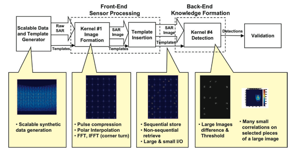
The precise algorithmic details of this particular SAR processing chain are given in its written specification. In Stage 1, the data is transformed in a series of steps from a n×mc single precision complex valued array to a m × nx single precision real valued array. At each step, either the rows or columns can be processed in parallel. This is sometimes referred to as “fine grain” parallelism. There is also pipeline or task parallelism that exploits the fact that each step in the pipeline can be performed in parallel, with each step processing a frame of data. Finally, there is also coarse grain parallelism, which exploits the fact that entirely separate SAR images can be processed independently. This is equivalent to setting up multiple pipelines.
At each step, the processing is along either the rows or the columns, which defines how much parallelism can be exploited. In addition, when the direction of parallelism switches from rows to columns or columns to rows, a transpose (or “cornerturn”) of the matrix must be performed. On a typical parallel computer a cornerturn requires every processor to talk to every other processor. These cornerturns often are natural boundaries along which to create different stages in a parallel pipeline. Thus, in Stage 1 there are four steps, which require three cornerturns. This is typical of most SAR systems.
In stage 2, pairs of images are compared to find the locations of new “targets.” In the case of the SAR benchmarks, these targets are just nfont × nfont images of rotated capital letters that have been randomly inserted into the SAR image. The Region Of Interest (ROI) around each target is then correlated with each possible letter and rotation to identify the precise letter, its rotation and location in the SAR image. The parallelism in this stage can be along the rows or columns or both, as long as enough overlapping edge data is kept on each processor to correctly do the correlations over the part of the SAR image for which it is responsible. These edge pixels are sometimes referred to as overlap, boundary, halo or guard cells. The input bandwidth is a key parameter in describing the overall performance requirements of the system. The input bandwidth (in samples/second) for each processing stage is given by
 (1)
(1)A simple approach for estimating the overall required processing rate is to multiply the input bandwidth by the number of operations per sample required. Looking at Table 1, if we assume n ≈ nx ≈ 8000 and mc ≈ nx ≈ 4000, the operations (or work) done on each sample can be approximated by
 (2)
(2)Thus, the performance goal is approximately
 (3)
(3)Tinput varies from system to system, but can easily be much less than a second, which yields large compute performance goals. Satisfying these performance goals often requires a parallel computing system.
The file IO requirements in “System Mode” or “IO Only Mode” are just as challenging. In this case the goal is read and write the files as quickly as possible. During Stage 1 a file system must read in large input files and write out large image files. Simultaneously, during Stage 2, the image files are selected at random and read in and then many very small “thumbnail” images around the targets are read out. This diversity of file sizes and the need for simultaneous read and write is very stressing often requires a parallel file system.
Table 1 provides a list of current implementations for each of the three SSCA benchmarks. The benchmarks have been implemented in several languages, with contributions from industry, academia, supercomputing centers and national labs.
Kepner and Meuse from MIT Lincoln Labs maintain the reference executable implementations inMatlab for the three SSCAs. Bader and Madduri have developed a parallel implementation of SSCA #2 in C using the POSIX thread library for commodity symmetric multiprocessors (SMPs). They evaluate the data layout choices and algorithmic design issues for each kernel, and also present execution time and benchmark validation results.17 Gilbert, Reinhardt and Shah describe a StarP implementation of SSCA #2 in [18]. The various SSCA implementations have also been compared for productivity studies.
| Benchmark Language | Bioinformatics (SSCA#1) | Graph Theory (SSCA#2) | Sensor and IO (SSCA#3) |
| Written spec | 0.5 (GT/LL) | 2.0 (GT/LL) | 0.8 (LL) |
| C | 0.5k1† (PSC) | 2.0 (GT) | 0.5 (ISI) |
| C & MPI | 0.5k1† (PSC) | ||
| C & MPI & OpenMP | |||
| UPC | 0.5k1† (UNM/GT/PSC) | 1.0* (UNM/GT) | |
| C & Pthreads | 0.5k1* (UNM/GT) | 2.0* (UNM/GT) | |
| C++ | 1.0 (LL/MITRE/CS) | ||
| Fortran | 2.0† (Sun) | 0.5io (LM) | Fortran & OpenMP | 2.0† (Sun) |
| Matlab | 0.5 (LL) | 2.0 (LL) | 0.8 (LL) |
| MatlabMPI | 1.0 (LL) | 0.8 (LL) | |
| Matlab & mexGA | 0.5* (OSC) | 1.0* (OSC) | 0.8* (LL) |
| StarP | 2.0* (UCSB) | 0.5 (UCSB) | |
| pMatlab | 1.0 (LL) | 1.0 (LL) | |
| Octave | 0.8* (OSC) | 1.0* (UW) | 0.8 (OSC) |
| Octave & mexGA | 0.8* (OSC) | 1.0* (OSC) | 0.5* (OSC) |
| Python | Python & MPI | ||
| Java | 0.5k1† (PSC) | 1.0int† (GT) | |
| Chapel | 0.5 (Cray) | 1.0int† (Cray) | |
| X10 | 0.5k1† (UNM/GT/PSC) | 1.0* (UNM/GT/IBM) | |
| Fortress | |||
|
CS: CodeSourcery, LLC GT: Georgia Institute of Technology ISI: Univ. of Southern California, Information Sciences Institute LL: MIT Lincoln Labs LM: Lockheed Matrin MITRE: MITRE Corporation OSC: Ohio Supercomputer Center PSC: Pittsburgh Supercomputer Center UCSB: Univ. of California, Santa Barbara UNM: Univ. of New Mexico UTK: Univ. of Tennessee UW: University of Wisconsin |
|||